Thanks for being with me so far. Just a few more steps before we can see our worksheet formatted to be reasonably presentable.
Let see what more needs to be done.
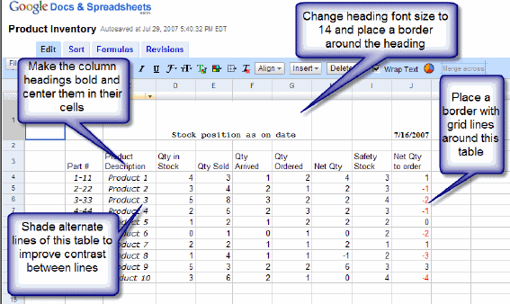
1. Change heading font size to 14 and place a border around the heading
Click on cell cell D1 to select the heading and click on the fontsize button on the tool bar. This drops down a set of available font sizes as shown below.
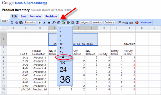
Select size 14 from this list by clicking on it.
Now to place a border around the heading, click on cell D1 again to select the heading. Click on Borders button (pointed by the arrow) on the tool bar. This drops down a list of available border styles. Select the first style from left on the top row.
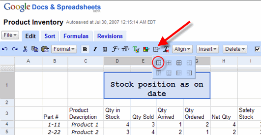
This surronds the heading with a border.
2. Make the column headings bold and center them in their cells
Click on cell B3 and hold shift key, and click on cell J3, to select all cells of the heading. Then click on bold button on the tool bar to make cell contents of cells B3 through J3.
Now click on Align button on the toolbar. This drops down a list of available options as shown below
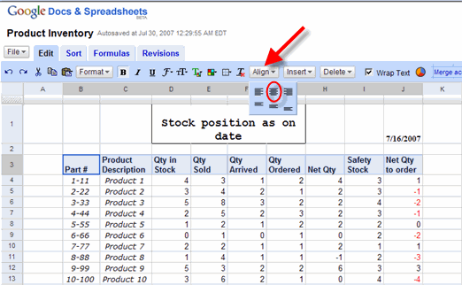
Choose center alignment by selecting the second from left on the top row.
3. Place a border with grid lines around this table
Click on cell B3 then hold the shift key and click in J13 to select the entire table.
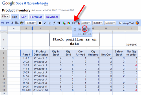
Now click on Borders button on the tool bar as pointed by the arrow. This drops down the available border styles. Choose the third from left on the top row.
4. Shade alternate lines of this table to improve contrast between lines.
Click on cell B5, hold shift key and click on cell J5 to select all cells B5 through J5. The entries in these cells correspond to Product 2.
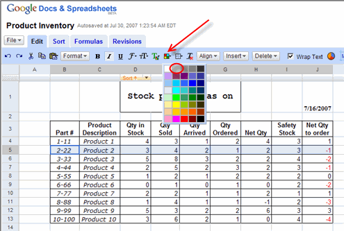
Now click on Background Color button on the tool bar as pointed by the arrow. This drops down the set of available colors to serve as background to selected cells. Select second from left on the topmost row (as shown cirled). This places all the selected cells with a grey background.
Repeat this procedure for entries corresponding to Products 4, 6, 8, and then 10. Now have alternate lines of the table with contrast as shown below.
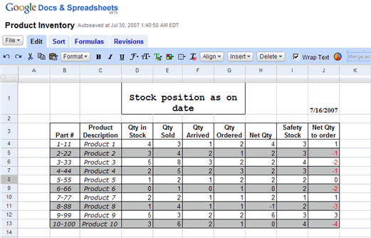
This completes the formatting of stocksheet.
<--BackTo: Format the worksheet I
Next: Format the Worksheet III –>