So far we have created a workbook with relevant data filled in and the appropriate documentation added. It is functional and informative. But it is not enough.
Though data is important, equally important is how it is presented to the viewer. It should be “user-friendly”, in the sense that
- it should be easy to understand.
- should make the viewer perceive the important elements of the spreadsheet.
- should be pleasing to the eye.
- finally impel him or her to take necessary action.
A little time spent in formatting the cell contents goes a long way towards meeting our objective.
There are two aspects to consider while formatting the cells:
1. how the cells appear : the cosmetic touch given to the cell contents like font size, alignment, coloring, typeface etc which make the overall spreadsheet pleasing to the eye.
2. how the cell values are displayed : this relates to formatting numbers, dates and time to suit the context and leave the viewer in clarity.
With this introduction, let us implement the following changes and see if it makes any difference.
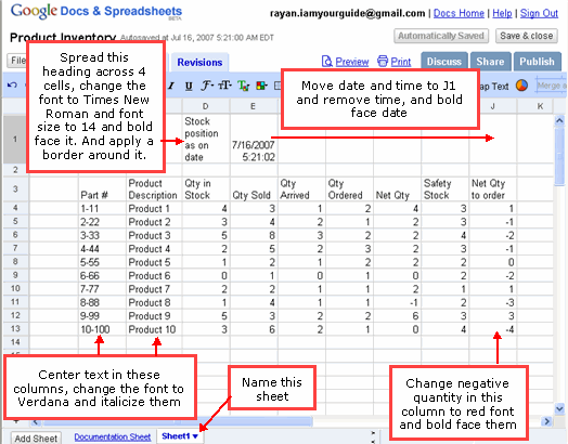
1. Center text in the first two columns, change the font to Verdana and italicize them.
Click on cell B4 and press and hold Shift key and click on cell C13 thus selecting cells B4 through C13.
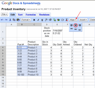
Click on the small inverted triangle on the Align button on the tool bar. This drops down several options to align the cell contents within the cells. Now choose the center alignment by clicking on the selection within the circle. This makes for the center alignment of all the cells B4 through C13.
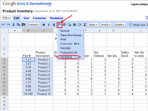
Now select cells B4 through C13 again as shown above, and then click on the font family button on the tool bar. This drops down a few fonts to select and now click on Verdana to select it as the appropriate font for these cells.
Finally to italicize these cells B4 through C13 , select them and click on Italic button on the tool bar as shown below.
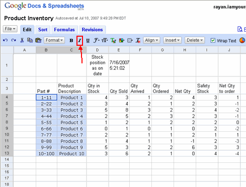
Now the cells B4 through C13 appear italicized.
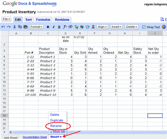
2. Rename this sheet (Sheet1) as “Stock Sheet” by clicking on the menu beside Sheet 1 and selecting Rename option.
3. To change the font color of cells in the column titled Net Qty to order, to red and bold face them.
Click on cell J5 and hold the left button and drag the mouse down to select cells J5 through J7. Click on text color button to display the available colors and then select red color pointed by the arrow. This converts cell contets in cells J5 through J7 to display in red.
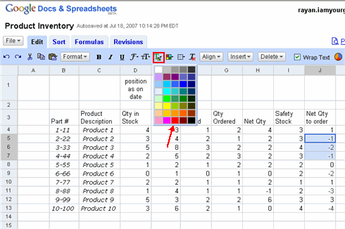
Apply similar procedure to display contents in cells J9, J11 and J13 in red by doing them one at a time.
4. Move date and time in cell E1 to cell J1, discard time and bold face date.
Rightclick on cell E1, and select Cut option
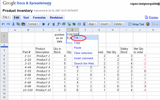
and then click on cell J1 and right click the mouse and choose the Paste date and time in this cell.
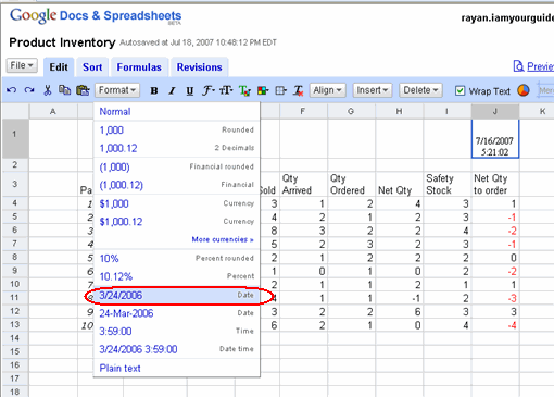
Click on cell J1 and click on Bold button in the tool bar to make the date as bold.
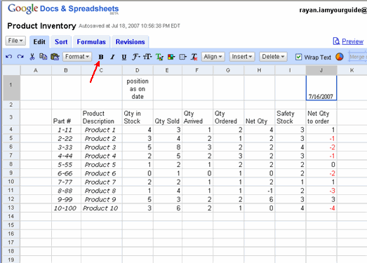
5. Now to spread the heading across 4 cells, change the font to Times New Roman and the font size to 14 and bold face it. And finally to apply a border around it.
Click on cell D1, and hold the Shift key and click on cell G1 to select all cells D1 through G1 and then click on Merge Across button on the tool bar.
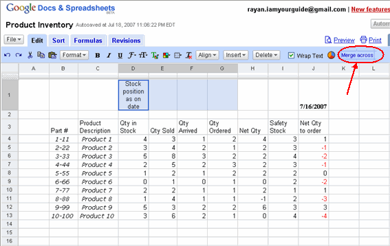
This spreads the heading across 4 cells. Now click on the heading and change the font to Times New Roman as we did above in step1, only this time choosing Times New Roman as our preferred font. And finally make it bold by clicking on Bold button on the toolbar as told above. The effect of these changes are as shown below.

Next: Format the Worksheet II –>