Here is the skeleton spreadsheet we made ready in the last session. 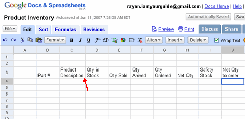
Now to start filling up the skeleton worksheet with data. In cell B4 type in 1-11 as part # for the first product, and press enter.
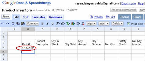
But as you could see the part # 1-11 is misread as a date January 11th 2007 by Google Spreadsheet. This is not our intention though. So to prevent such automatic interpretation, we need to precede our entry with a single quote ” ‘ “. This way it would be exactly as we intended it to be. So click on cell B4 and type a single quote ‘ followed by the part # 1-11 like ‘1-11 and the press enter.
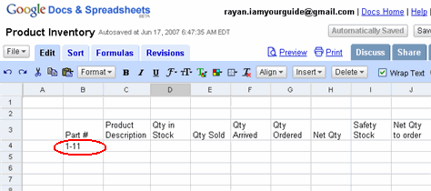
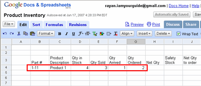
Now you could see that the part is correctly entered. Click on C4, type in Product 1 and press tab to move the pointer to cell D4 and type in 4 for Qty in Stock. Press tab again to move over to cell E4 and type in 3 for Qty Sold. Like wise move over to cells F4 and G4 and type in 1 and 2 for Qty Arrived and Qty Ordered respectively. As of now the cell entries should look like the figure shown below. If there are any differences please correct them now, before we proceed further.
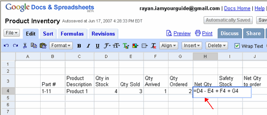
Now we are ready to enter the formula for calculating the Net Qty in cell H4. Remember our formula for Net Qty (Net Quantity) = Qty in stock – Qty Sold + Qty Arrived + Qty Ordered. So click on cell H4 and type in the sign = ( to signify that it is a formula), followed by D4 – E4 + F4 + G4 and press enter. If in doubt please see the entry below. The answer 4 appears in cell H4.
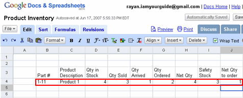
Click I4 to enter the Safety Stock. Type in 3 in this cell for safety stock and press tab key to move over to cell J4. Previous session you know that the formula for Net Quantity to order (Net Qty to order) = Net Quantity – Safety Stock. So we type in cell J4, = H4 – I4 and press Enter. All the entries for Product 1 are now completed and should look like the picture shown below.
Fill in the data for part #, Product Description, Qty in Stock, Qty Sold, Qty Arrived, Qty Ordered and the Safety Stock for the balance 9 products as shown below. Please remember when you enter the part #, it needs to be preceded by a single quote ” ‘ “.
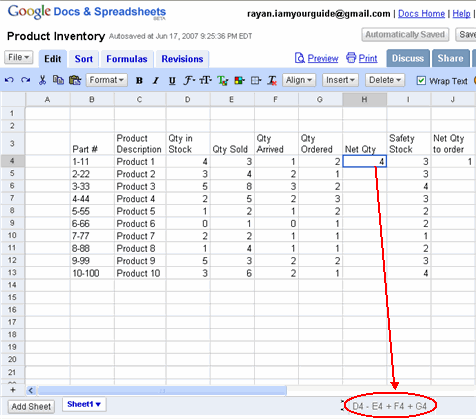
Please note that only the columns Net Qty & Net Qty to order are remaining to be filled. These are derived figures from formulas and we can either enter the formula for each cell or we can copy the formulas from the first line and paste in the rest of the cells in a particular column. We will take the easier route of copying and pasting the formula. For instance for cell H4, the formula is = D4 – E4 + F4 + G4 ( this is seen at the bottom when we click on cell H4) and this can be copied and pasted in cells H5 through H13.
The procedure is as follows:
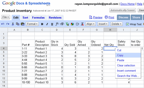
Click on cell H4 and right click and select copy. See picture below for details:
Select cells H5 through H13, by clicking on cell H5, and holding the Shift key while simultaneously clicking on cell H13. Once these cells are selected, right click on them and select paste as shown below.
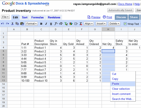
After pasting the formula, the entries appear for the Net Qty in column H as shown below.
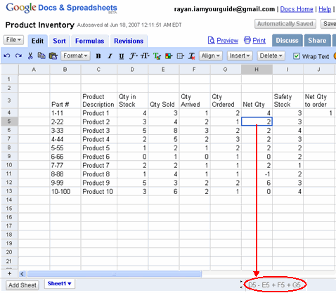
As is seen above the formula is copied down the line. For instance when we click on H5 the value in cell H5 (the Net Qty) is derived from the formula = D5-E5+F5+G5 which is ( = Qty in Stock – Qty Sold + Qty Arrived + Qty Ordered and in numerically it is = 3-4+2+1 giving us the result 2 for Net Qty) exactly what we want for Product 2.
Finally we need to find out Net Qty to order for the balance 9 products. For this we can copy and paste the formula like we did above. But this time we copy the formula from cell Net Qty to order. So click on cell J4 to select it, then right click on it, from the sub menu click on copy, to copy the formula. Now click on cell J5, press and hold Shift key, and simultaneously click on cell J13. This selects cells J5 through J13. Now right click on any one of the selected cells, and choose paste from the submenu that appears. This pastes the formula for all the cells J5 through J13.
Your completed table should look like the one shown below.
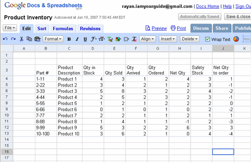
Remember our rule for ordering, only those that are negative in the column Net Qty to order need to be ordered. So we see that Products 2, 3,4 and Products 6, 8 and Product 10 only need to be ordered as per the quantity listed in this column.
<--BackTo: Create a skeleton worksheet