Your completed list will look like the one shown below. ( Just to remind ourselves the terms record and fields, I have super imposed these on the list. In your list these may not appear. So don’t worry) :
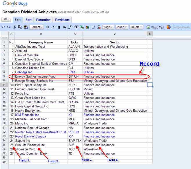
Now with this list before us we can do some basic list manipulations:
1. Freeze header rows:
Some times we are not able to see the entire list ( if the list is too long to be accommodated within the computer screen).
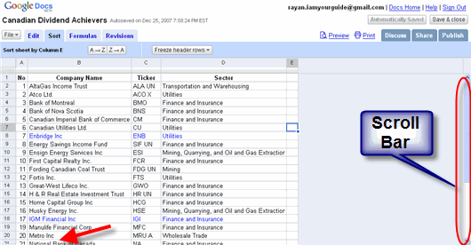
We need to scroll down (using scroll bar on the side) the list to see companies listed right at the very bottom. That is ok but look what happens when we scroll down.
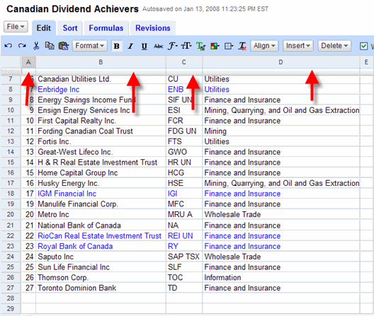
Ofcourse we can see the bottom of the list. But where are the headings? The header row is now hidden at the top as pointed by the arrows. It is important to know the field names in the header to relate them to the values in the list.
In order to preserve the header row and keep it in visibility, while we scroll down a long list, we can freeze it using the following procedure. First use the scroll bar all the way up so that the header comes into picture as shown below. Then click on the sort tab to make the ‘Freeze header rows’ option becomes accessible.
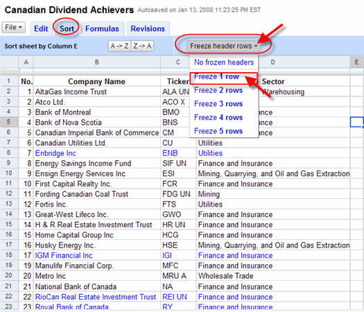
Now click on the small drop down arrow beside the Freeze header rows to see the drop down list. In the drop down list you see that you can freeze 1 row to as many as 5 rows.
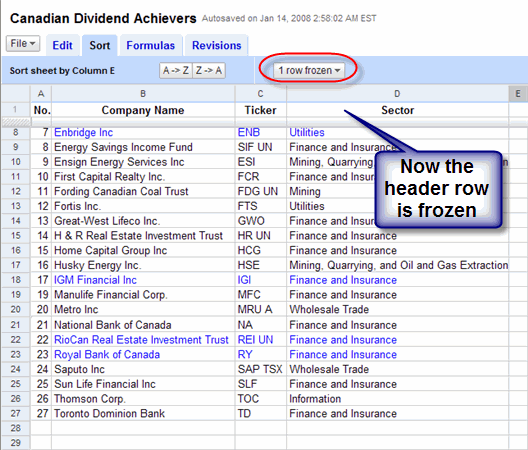
Our header row needs just 1 row to be frozen, so we select that and the header row now stands frozen. We can see all the column headings even we scroll down to the very bottom of the list.
2. Sort on a particular field ( say Filed 2 – Company name)
Often times we may come across the need to sort on a particular field to quickly see for we are looking for.
If you see currently the list is sorted on company name in an alphabetical order A -> Z. i.e. The name AltasGas Income Trust appears first and Toronto Dominion Bank appears last.
We can reverse this order by sorting on the field Company name.
If you remember we discussed briefly about sort options in Chapter 1 Introduction to Google Spreadsheets under the section Google Spreadsheet Window.
Now we are going to make practical use of it. Click on sort tab and click on column B to select the entire column as shown below:
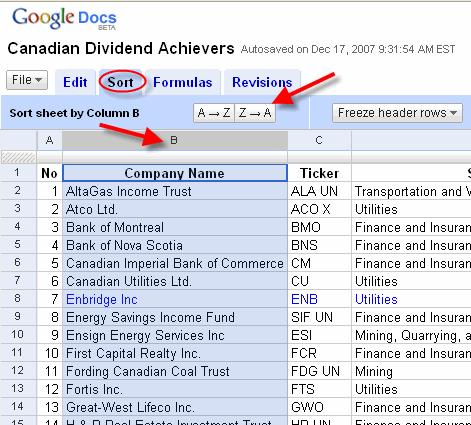
Finally click on the button Z -> A to reverse the order as shown below:
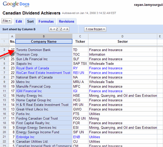
Now as you can see Toronto Dominion Bank comes out on top. Click anywhere within the spreadsheet to deselect the column B as you may not want it be affected if you choose to do something else with the spread sheet.
<--BackTo: Planning and creating a list